A finite/boundary element study using Comsol Multiphysics

Andrew Watson (December 2021)

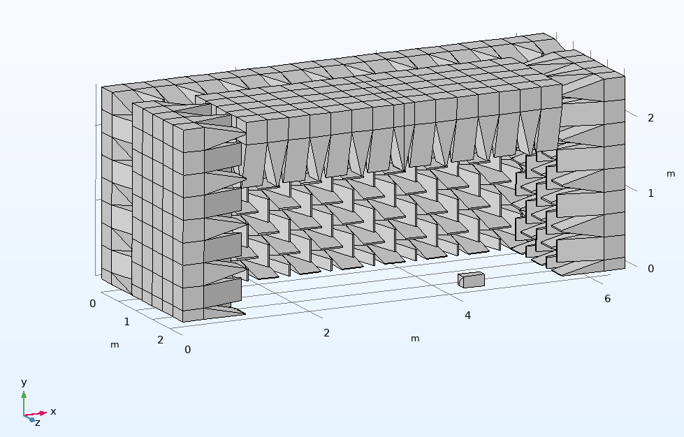
Figure (1a) Geometry of the chamber simulation (quarter model).

Introduction

Anechoic chambers are commonly used for the measurement of loudspeakers. They provide a ‘free-field’ environment devoid of any reflections that could interfere with the direct signal from loudspeaker to microphone.

The walls of the chamber are covered with sound absorbing material, typically wedge-shaped blocks of foam or fibreglass which provide a gradual transition from air to solid absorbent. The useable, anechoic measurement region, is generally regarded as being a wedge’s length in from the wedge tips.

The length of the wedges is critical in determining the low frequency limit for anechoic behaviour. It is normally stated that the chamber is anechoic down to the frequency where the wedge length is one quarter of a wavelength. So, for example, 90cm wedges can provide anechoic performance down to around 95Hz. However, to achieve this cut-off in practice may require the speaker to microphone axis to be carefully positioned within the chamber.

It is sensible to choose the dimensions of the chamber so as to provide an even spread of the room modes. Coincident or closely spaced modes may result in non-anechoic behaviour to well above the nominal cut off frequency. The dimensions of the chamber should ideally be chosen as if one was designing a listening room.

The practical anechoic cut off frequency will also depend on the measurement distance. For example, increasing the measuring distance from 1m to 2m in a given chamber will reduce the level of the direct signal relative to the non-absorbed chamber signal by approximately 6dB. This may significantly increase the cut-off frequency.

The effect of non-anechoic chamber behaviour on the measured response

If one measures a loudspeaker in a typical anechoic chamber the measured response will be accurate above the anechoic cut-off frequency, but will show increasing error below this due to the progressively decreasing absorption of the wedges. However, this error can be quantified and a correction curve can be generated for loudspeaker measurements.

Derivation of a chamber correction curve.

For a given loudspeaker, if its measured response in the chamber is divided by a free-field response of the speaker on the same axis (with corrections made for any environmental differences), one has a chamber correction curve for that speaker. This correction curve will be specific to the chosen source and receiver locations within the chamber and, strictly speaking, this curve will be specific to that speaker size and format.

The concept of anechoic chamber correction curves for loudspeaker measurements has been around for many years. The author was introduced to them back in 1994 on joining KEF Audio, where it had been established¹ that, for that particular chamber and its measurement geometry, one correction curve sufficed for a range of typical speaker sizes. The author used this chamber extensively in the measurement of loudspeakers and also studied different ways of generating correction curves such as the far-field/nearfield technique described below. The purpose of this article is to use finite and boundary element modelling to take a more general view of chamber correction curves.

Modelling the anechoic chamber

A finite element (pressure acoustics) model of a medium-sized anechoic chamber, suitable for 2m measurements, has been written in Comsol to simulate the process of generating correction curves. The dimensions are 6.3m(L) x 5.1m(H) x 4.8m(W) with wedges of 90cm total length and 30x30x30cm base. The acoustical properties of the wedges are modelled, using the poro-acoustics function, as a material with a flow resistivity of 5000 mks rayls/m, using the Delany and Bazley model with standard constant values. The wedges are assumed to be a rigid porous medium – structural motion in the wedges is not modelled in this study. The chamber walls are assumed to be rigid and there is no door. The measurement axis is along the centre line of the long dimension (for symmetry and to facilitate a faster running quarter-model of the chamber) with the microphone at L=2m and the speaker baffle at L=4m. The Comsol model geometry is shown above in figure (1a) with the schematic in figure (1b).

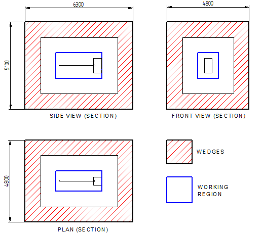
Figure (1b) Schematic of the modelled chamber.

Four monopole test loudspeakers are modelled: (1) a 2” size – 4cm diameter circular piston on the front of a 6 x 6 x 6cm rigid box, (2) a 6” size – 13cm piston on the front of an 18 x 18 x 18cm box, (3) a 10” size – 25cm piston on the front of a 30 x 30 x 30cm box and (4) a 15” size – 32cm piston on the front of a 45 x 45 x 45cm box. The pistons are assigned a constant acceleration with frequency. The free field responses of these four speakers are simulated with a boundary element model. Figure (2) shows the chamber correction curves generated with these four speakers. As all the speakers are mounted with their baffles at L=4m we can call these ‘co-planar’ correction curves.

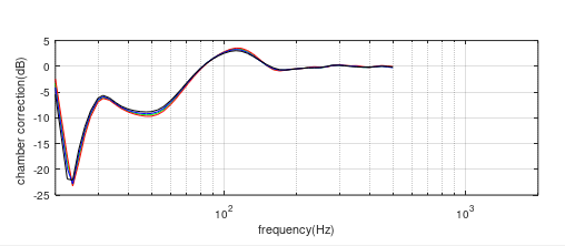
Figure (2) Co-planar chamber correction curves generated from chamber response/free field response for 4 monopole loudspeakers. Red = 2”, Green = 6”, Blue = 10”, Black = 15”.

The first thing one notices about this result is that the four correction curves are very similar, particularly the 6, 10 and 15”. The chamber’s influence on the measured response extends up to around 220Hz.

Source centres

By studying the polar responses of the free-field boundary element simulations the effective source centres of the test speakers – the centre of spherical radiation - can be estimated, figure (3). For these test speakers these turn out to be in front of the baffle by 2.4cm for the 2” box, 7cm for the 6” box, 12cm for the 10” and 18cm for the 15”. The present simulations define flat piston radiators, but the result holds also for conical radiators. An approximate formula for estimating the distance between the baffle and the effective source centre is 0.8 x (H x W) / (H + W).

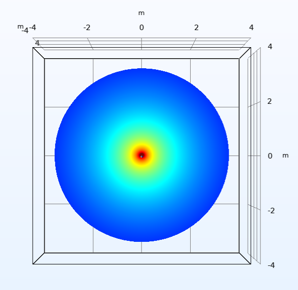
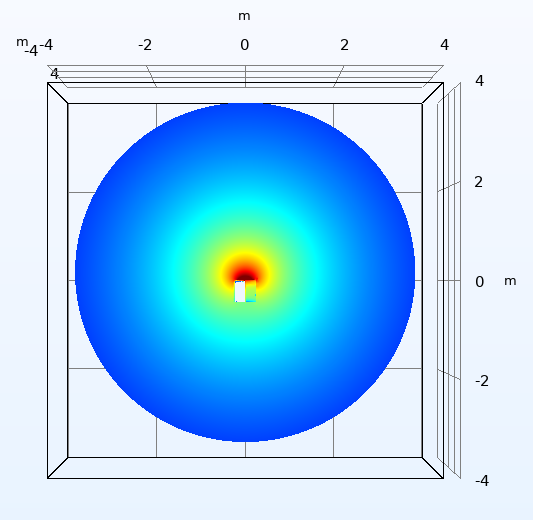
Figure (3) Polar patterns at 20Hz for the 2”(left) and 15”(right) test speakers with their baffles at L=4m.

The simulations can then be re-run with each speaker moved back to place their effective sources centres at the L=4 position, -2.4cm for the 2”, -7cm for the 6”, -12cm for the 10” and -18cm for the 15” speaker. The four new correction curves are shown in figure (4) and are now significantly closer to each other. A difference curve between the 2” and 15” speakers is shown in figure (5) and confirms that they are within 0.5dB of each other above 25Hz. This shows the importance of the effective source location on the chamber response.

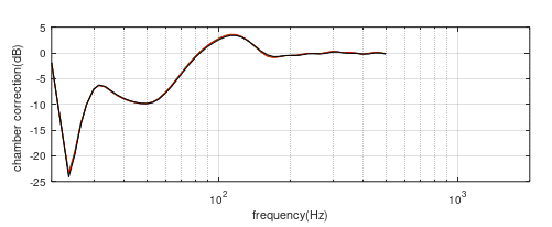
Figure (4) Chamber correction curves generated from chamber response/free field response for the four test speakers with their effective source centres coincident. Red = 2”, Green = 6”, Blue = 10”, Black = 15”.

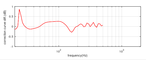
Figure (5) Difference between the 2” and 15” chamber correction curves when their effective sources are coincident.

So, with knowledge of, or a good estimation of, the effective source centre the same correction curve can be used with a range of speaker sizes with good accuracy and uniformity. This will require that the different sized speakers have to be positioned at different distances from the microphone and a correction made to the sensitivity calculation. Alternatively, the speakers can all be measured co-planar with the baffles at L=4, and with reference to the results in figure (2) an average correction curve of the practical baffle sizes (6” to 15”) can be made which will give a correction to an accuracy of better than +/-0.75dB above 28Hz, figure (6).

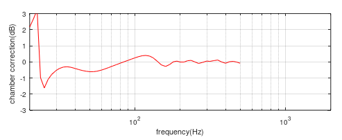
Figure 6) Difference between the 6” and 15” chamber correction curves when their baffles are co-planar at L=4m.

Now let us consider some factors which could potentially affect the correction curves.

At the upper end of the chamber response, around 100-220Hz, any differences between the correction curves may be due to the different directivities of the four speakers. Figure (7) shows this for all four speakers at 200Hz, looking down onto the speakers with the microphone towards the top of each graph. The 2 and 6” speakers are clearly very close to omni-directional, the 10” is clearly closer to omni- than uni-directional and the 15” is maybe half way in between. However, for this chamber configuration and the 2m measuring distance, the 15” co-planar correction curve, above 30Hz, is still within 1dB of that of the 2”. This suggests that at these frequencies (150-220Hz) the forward radiation, where the polar patterns are quite similar, is more important than the rearward.

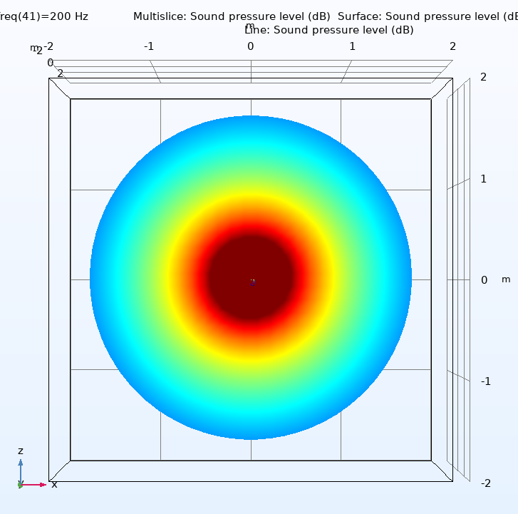
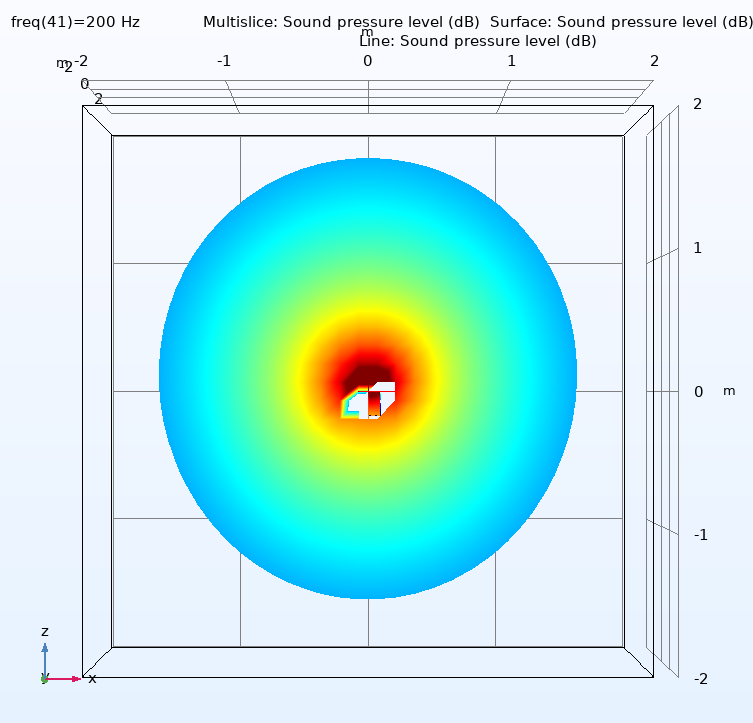
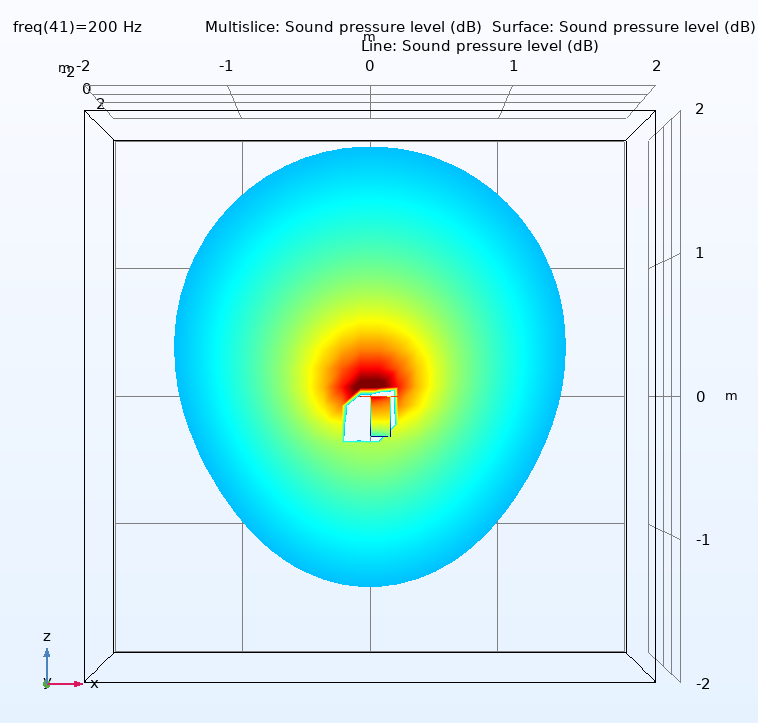
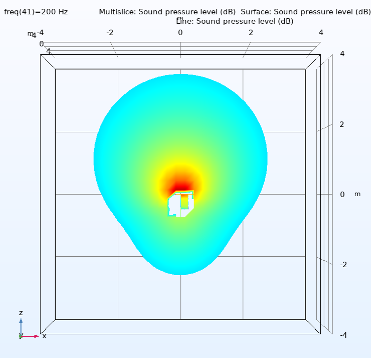
Figure (7) Polar responses of the four test loudspeakers at 200Hz. Top left: 2”, Top right: 6”, Bottom left 10”, Bottom right 15”.

An alternative way to compare the directivities of the four speakers is to look at the free field responses in the far-field which illustrate the well-known 4pi (omni-) to 2pi (uni-directional) transition, figure (8). The pistons move with constant acceleration and would thus produce a flat response at 0dB when mounted in a 2pi baffle. In the low frequency (omni) region the curves tend to -6dB (as half the sound energy is now going backwards), and in the uni-directional region the response stays at 0dB (with some peaks and dips due to box edge diffraction) The measuring distance of 10m ensures that we are looking at the close to the true far-field response.

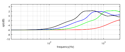
Figure (8) Free field responses of the four loudspeakers at 10m distance. Red=2”, Green=6”, Blue=10”, Black=15”.

At 100Hz, all four speakers are either omni or very close to omni. The biggest differences in the directivities are between 200 and 700Hz. At 400Hz, for example, the 2” speaker is very close to omni- and the 15” is predominantly uni-directional. However, above 200Hz the chamber is fully anechoic and all off-axis radiation is fully absorbed by the wedges. This helps to explain why the correction curves for the four speaker sizes are so similar.

At the very low frequencies the modal behaviour of the chamber becomes apparent as the absorption of the wedges progressively reduces. In this region, differences between the correction curves, aside from the source centres and their influence on the room modes, may be due to the proximity of the outer edges of the larger boxes to the rear and side wedges.

From observation of the free-field BE simulated data, for the 6” speaker, spherical radiation to the rear will be happening from about 0.5m from the back of the speaker, which for the modelled chamber, is well before it reaches the wedges. For the larger speakers, though, the complex nearfield region around the speaker means that spherical radiation only appears to form at distances greater than about 1m from the back of the speaker. If the wedge tips are less than 1m from the back of the speaker then they will be receiving a somewhat non-spherical wave front shape.

Discrepancies between the curves at the low frequencies can be investigated by looking at the pressure distributions in the chamber at those frequencies. Figures (9a) and (9b) below show this for the 2” and 15” cabinets at 30Hz.

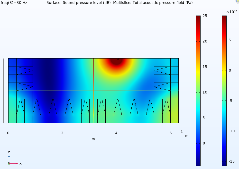
Figure (9a) Sound pressure level in the chamber at 30Hz for the 2” speaker at L=4.024m.

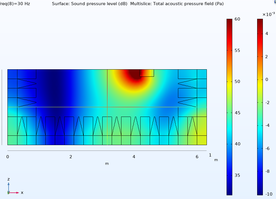
Figure (9b) Sound pressure level in the chamber at 30Hz for the 15” speaker at L=4.18m.

With the source centres coincident the modal behaviour in the room is very similar but one can detect small differences between the back of the speakers and the rear wedges. This may become a problem if the default speaker location is too close to the rear wedges.

Obtaining a free-field measurement of a test loudspeaker

A free-field response of the speaker can be done in a number of ways such as outdoor measurements, a combination of cone excursion (or nearfield pressure) measurement and boundary element simulation or signal conditioned indoor transient measurements¹.

Chamber correction using the far-field/near-field method².

The primary assumption of this method is that the correction curve is derived for monopole, omni-directional radiation, and, as will be discussed below, for most setup conditions this can suffice for a wide range of speaker sizes. This method can be used when there is no free-field measurement of the test speaker(s). In the following description we first consider co-planar baffles and then later we shall deal with coincident effective sources. The method uses test speakers of different sizes. With reference to the data in figure (8) we can specify a strict upper limit of omni-directional behaviour as the frequency where the curves reach -6 + 0.25dB. This gives us 70Hz for the 15”, 105Hz for the 10”, 170Hz for the 6” and 500Hz for the 2”.

Firstly, a very small system comprising a 2” or 3” unit mounted in a small box or in the end of a rigid tube (approximately 50cm long - for ease of mounting). The criterion for this speaker is that it should be omnidirectional to well above the cut off frequency of the chamber. It is placed in the standard source position and measured firstly at the designated measurement point (the far-field) and then in the nearfield. (Note that nearfield measurements of such small units should be done with a quarter-inch sized microphone).

At the low frequencies, where the speaker is omnidirectional, the shape of nearfield and far-field responses is the same³. Dividing the far-field by the near-field responses produces the first correction curve, figure (10). This is shown (in red) compared to the previously derived 2” correction curve (in blue) from figure (2). This confirms the equivalence of the nearfield and far-field curves in the speaker’s omnidirectional range. Below the chamber cut off frequency (220Hz) the correction curve will show the chamber response. At frequencies immediately above this the curve should be flat – the chamber is anechoic here and the speaker is still omnidirectional – this flat region allows one to define the 0dB level of the correction curve - the curve is level adjusted until the average level in the flat region is 0dB. As the frequency increases further one sees the curve gradually rise due to the speaker becoming directional. At a suitable zero-crossing point the curve can be set to 0dB for all higher frequencies – where the chamber is anechoic and there is no need for any correction.

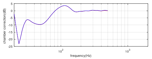
Figure (10) 2” chamber correction curves. Red = 2m far-field (chamber) divided by nearfield (chamber), Blue = 2m far-field (chamber) divided by 2m far-field (free-field).

Larger speakers, such as a 6”, 10” and 15” size, can then be measured in the same way to produce further correction curves, with progressively better signal to noise ratio at the lower frequencies. As was shown above, the shape of these curves should be very similar to the 2” curve and should be level matched to that. First, the 6” curve is level is matched to the 2”, figure (11) between an upper frequency limit, which defines the onset of the larger system’s box directivity and a lower limit which defines where the curves deviate at the lower frequencies due to the effective source position being different (refer to figure (2)).

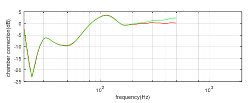
Figure (11a) Far-field/nearfield correction curves. Red = 2”, Green = 6”

Next, the 10” curve is level matched to the 6”, figure (11b), and then the 15” is matched to the 10”, figure (11c). The overlay of all four curves is shown in figure (11d).

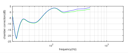
Figure(11b) Far-field/nearfield correction curves. Green = 6”. Blue = 10”.

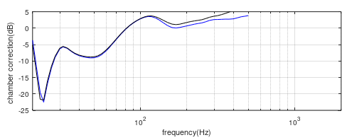
Figure(11c) Far-field/nearfield correction curves. Blue = 10”, Black = 15”.

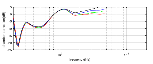
Figure (11d) Chamber correction curves based on far-field divided by nearfield measurements. Red: 2” speaker, green: 6”, blue: 10”, black: 15”.

From this set of overlayed curves one can decide whether separate curves are needed for different sized boxes or whether – as in this case – one curve will suffice.

We can now produce a compound correction curve by splicing together the data from the four level matched test boxes at appropriate frequencies. This must include the 2” curve at the higher frequencies as this defines the 0dB level and, at the lower frequencies, the choice is based on (1) which of the larger units best represents the average speaker size and (2) which have an adequate signal to noise ratio for the data to be reliable down to the lowest frequency of interest. The choice of a third intermediate curve such as the 6” will depend on whether it provides necessary continuity.

The final curve will be made by splicing together two or more of these curves – such as the 10” and 2” at 100Hz, figure (11e). Again, providing that their correction curves are only used in the respective driver’s omnidirectional range. We now have a chamber correction curve for co-planar speakers which is optimised for the 10” baffle size (and effective source centre).

Note that when performing the far-field/nearfield division the nearfield curve should be time aligned with the far-field to maintain proper phase relationships, and then both aligned for zero delay before being applied to measured data. Also, we need to remember that we have chosen the 10” curve below 100Hz for which the effective source centre is 12cm in front of the standard baffle location, that is, at L=3.88m.

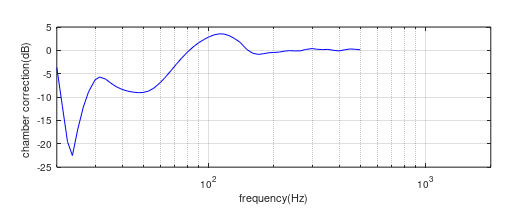
Figure (11e) Final chamber correction curve – 10” and 2” curves level matched and spliced together at 100Hz.

Deriving a far-field/nearfield correction curve for coincident sources

Although the speakers have to be carefully positioned so that their effective source centres are at the same point, the level matching process should be significantly easier as the shape of the curves should be more similar (from figure (4)). If we define the correction curve source centre as being that of the 10” speaker (the closest to average speaker size) when the baffle is at L=4m then the 2” speaker should be measured at L = 4 - (0.12 – 0.024) = 3.904m, the 6” at L = 4 - (0.12 – 0.07) = 3.95m, and the 15” at L = 4 - (0.12 – 0.18) = 4.06m. The level matching and splicing process can then be done as before to create a coincident chamber correction curve with the effective source centre defined at L=3.88m.

Figure (11f) shows the overlay of the 10” and 2” far-field/nearfield correction curves with the 2” unit 9.6cm forward to align the effective source centres. The match at the low frequencies is much closer than before, making the level matching process significantly easier. These two curves are again spliced together at 100Hz to create the coincident chamber correction curve, figure (11g), shown as an overlay with the coplanar curve.

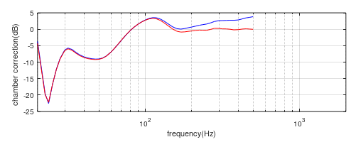
Figure (11f) Comparison of coincident far-field/nearfield correction curves for the 10” (blue) and 2” (red) test speakers at L=4m and L=3.904m.

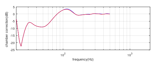
Figure (11g) Comparison of coincident (red) and coplanar (blue) chamber correction curves.

As expected, they are the same below 100Hz because they both use the 10” speaker measured at L=4, but slightly different between 100 and 150Hz – this is the effect of moving the 2” unit forwards by 9.6cm to align the effective source centres. The coincident effective source method is preferred for both accuracy and ease of derivation.

We then have the option of a using the co-planar or coincident correction curves, with the baffles at L=4m and optimised for the 10” speaker size or, if we need equal accuracy for larger or smaller speaker sizes, they can be positioned closer or further away from the microphone to align the effective source centre with that of the correction curve, and a sensitivity adjustment made.

Now let us consider some different loudspeaker formats and whether the correction curve thus derived will suffice for those.

(1) Twin 10” LF floor-standing speaker. This example has dimensions 1m(H) x 0.3m(W) x 0.3m(D) with two 25cm (10”) pistons positioned with their centres 16cm above and below the vertical mid-point of the front baffle. The speaker height is set so that the vertical midpoint of the cabinet is at microphone height. The chamber/free-field correction curve is shown in figure (12) along with the coincident chamber correction curve.

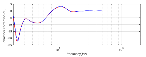
Figure (12) Chamber correction curve generated from a twin 10” piston tower speaker. Blue=coincident chamber correction curve, Red=twin piston correction curve.

The match is very good with a slight variance around 50Hz and 100Hz. The effective source centre for this speaker has been determined as 17cm in front of the baffle compared to the 12cm of the 10” speaker from which the correction curve is based. Figure (13) shows the same for the speaker moved back in the chamber by 5cm.

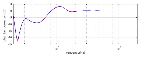
Figure (13) Chamber correction curve generated from a twin 10” piston tower speaker with baffle at L=4.05m. Blue=coincident chamber correction curve, Red=twin piston correction curve.

Here the agreement is even better, showing the significance of precise location of the source centre.

(2) Twin 10” LF floor-standing speaker measured at tweeter height. Let us now consider a typical measurement scenario when a typical floor-standing speaker 0.3(w) x 0.3(D) x 1m(H) with two 250mm pistons is first measured at tweeter height. The centre-point of the two pistons is -0.5m below the microphone height. A half-model is used in this simulation, figure (14).

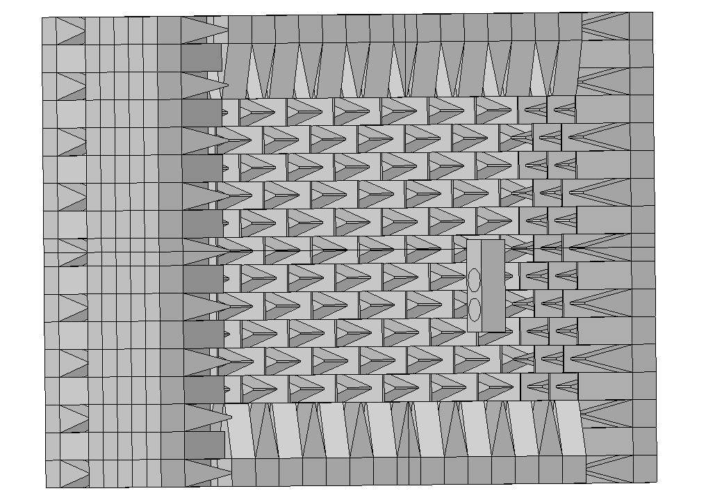
Figure (14) Half-model of the twin LF floor-stander measured at tweeter height.

The chamber/free-field correction curve for the LF system in this location is shown in figure (15) again compared to the coincident correction curve.

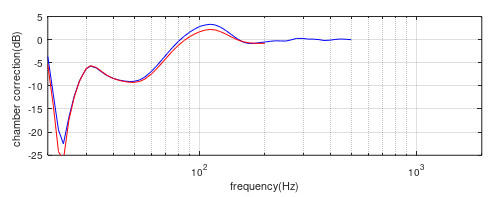
Figure (15) Chamber/free-field curve for the twin LF system lower by -0.5m (red) compared to the coincident chamber correction curve (Blue).

Here we see that the correction curve for this configuration is within approximately 1dB of the standard coincident correction curve above 25Hz meaning that, aside from the region below 25Hz and the deviation of around 1.25dB around 100Hz, the free field response of the whole system is determined with reasonable accuracy at the 2m on-(tweeter)-axis measuring position. For a more accurate measurement of the LF system alone, one would raise the speaker so that the LF vertical mid-point is at microphone height (and/or shift the speaker backwards by 5cm to align the effective source centre with that of the correction curve), as in figures (12,13). However, it is very useful to have a single accurate wide-band measurement of a system of this type on the listening axis (approximately tweeter height), without having to synthesise a system response from separate measurements and this would be an instance of where a separate correction curve is merited.

(3) Side firing pistons. The standard 10”, 30 x 30 x 30cm, test box now has two 25cm pistons mounted centrally on the sides. Initially, the front baffle is in the standard position (L=4m). The chamber/free-field correction curve based on this format is shown below in figure (16), again compared to the coincident chamber correction curve.

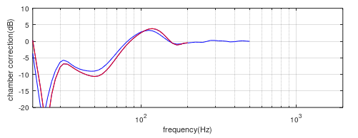
Figure (16) Chamber/free-field correction curve for 10” side firing pistons (red) compared to the coincident chamber correction curve (blue). Baffle at L=4m.

Here we see a significant difference between the two curves. This is also due to the effective source location now being 15cm further back from the front baffle, as well as 12cm back from the source centre of the standard correction curve. To investigate this, the next model has the speaker moved forward by 27cm (15 + 12cm) so the source centre is now at L=3.88m, figure (17), to match the source centre of the 10” test speaker.

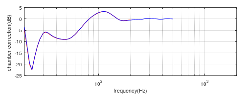
Figure (17) Chamber/free-field correction curve for 10” side firing pistons (red) compared to the coincident chamber correction curve (blue). Baffle at L=3.73m.

The agreement is now much better, again showing the importance of placing the speaker such that the centre of low frequency radiation is coincident with the designated source location used in the derivation of the standard correction curve.

(4) Rear firing piston. The piston on the standard 10” test box is now moved to the rear surface and the speaker is moved such that the rear face is at L=3.76m – 24 cm (2x12cm) forward of the front baffle of the forward-facing test box. The chamber/free-field correction curve for this rear facing speaker is shown in figure (18). Here we have a perfect match to the coincident correction curve.

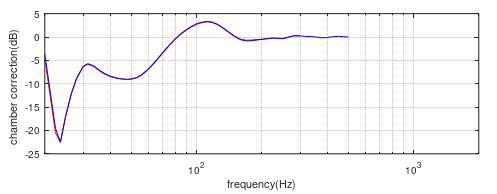
Figure (18) Chamber/free-field correction curve for the 10” test box with rear firing piston (red) compared to the coincident chamber correction curve (blue). Baffle at L=3.76m.

(5) 15” rear firing speaker. Here, the standard 15” test speaker is positioned with the piston on the rear face and with that face at L=3.64m (4 – 2 x 0.18). This places the effective source centre in the same position as that of the forward firing 15” speaker with baffle at L=4m – the two chamber/free-field correction curves are compared in figure (19).

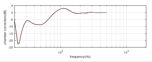
Figure (19) Chamber/free-field correction curves for the 15” forward and rear firing speakers with source centres coincident at L=3.82m. Red = rear firing, black = forward firing.

In this situation the directivity patterns relative to the measurement axis, as with the rear firing 10” example above, are reversed and the correction curves are the same. However, subtracting the direct signal from the total chamber response shows a correlation between the chamber response alone and the direct signal suggesting that the forward radiation (towards the microphone) is more significant, figure (20). This is reasonable as (although a ray tracing analysis should be used with caution in this instance) the forward radiation will produce the first (and loudest) reflections to arrive at the microphone. It is worth noting how the chamber responses deviate at around 220Hz – this would appear to be where the effects of the opposite directivities appear in the data. However, at this point the chamber-only response is more than 20dB below the direct signal and hence this does not affect the correction curve.

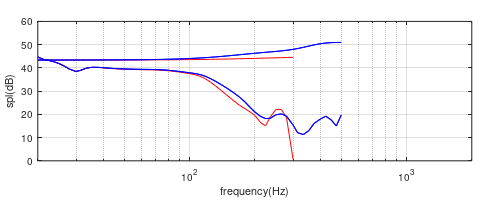
Figure (20) 15 inch forward and rearward firing test speaker with effective sources coincident. Upper curve is the free-field response, lower curve is chamber response only (total chamber response minus free-field). Blue = forward firing, Red = rearward-firing.

Dipoles

Now we shall consider what happens when we test a speaker with a markedly different source characteristics to that of a monopole. The correction curves for two dipoles have been simulated in figure (21). The first is a 1m x 1m baffle with a depth of 0.1m with two 250mm (10”) pistons positioned centrally on the front and back surfaces operating in dipole mode. The second comprises two 130mm (6”) pistons on a 0.5 x 0.5 x 0.1m baffle. The two baffles are mounted with the baffle fronts at L=4m and the unit centres at microphone height. The two chamber/free-field correction curves are very similar to each other and have an overall similarity with the standard (monopole) correction curve but the magnitude of the correction is much less. Clearly the chamber response is markedly different to that in the case of monopoles, this will mainly be due to the different way in which the dipole excites the modal behaviour of the chamber.

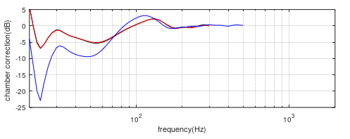
Figure (21). Comparison of the standard coplanar (monopole) correction curve (blue) with the 0.5m (red) and 1m (black) dipole chamber/free-field correction curves.

Conclusions

In this article we have seen that, for a sensibly designed anechoic chamber, the generation of correction curves is straightforward and it is likely that one curve will suffice for a range of loudspeaker sizes and formats. The importance of the effective source location is emphasised in relation to obtaining high levels of accuracy.

The far-field/near-field method allows the determination of a correction curve when true free field measurements of the test speakers are not available.

The above analysis is based on a chamber design that is built around a 2m measuring distance, is not constrained in any particular dimension and the nominal working region around the speaker and microphone is not compromised. Sometimes, though, one has to make compromises based on available space or cost and this can lead to the performance being limited in some areas, typically causing an increase in the anechoic cut-off frequency. This may bring directivity or other effects into play with regard to chamber correction and limit the range of speaker sizes that can be covered by a single correction curve.

References

[1] At KEF in 1993/4, the BDC (bass diminishing circuit) technique was used to obtain the true free-field responses of three speaker sizes – bookshelf, small floor-stander and large floor-stander when measured in the large transient room. The resulting three (1m) chamber correction curves were very similar allowing one to be selected for general use.

[2] The far-field/near-field technique was developed in 1998 by the author while also working at KEF.

[3] Keele, D.B. Low frequency loudspeaker assessment by nearfield sound pressure measurement. JAES, Vol.22 Issue 3, 154-162, 1974.

Contact: Dr Andrew Watson, Stonegate Acoustics Ltd, info@stonegateacoustics.co.uk